TensorFlow and Swift

Nov 17, 2018 in ADVANCED • EDGE AI • S4TF • SWIFT • TENSORFLOW
24 min read

Video / Slides

Introduction (0:00)

We’ll talk about TensorFlow and Swift today. Earlier this year, I went to the TensorFlow Dev summit, where Google announced TensorFlow for Swift, and then TensorFlow.js. A couple weeks later, Chris Fregly invited me to come to his Spark and TensorFlow meet up and talk about TensorFlow.js. I was going to make some demos, but my speech mutated into why you would even want to use JavaScript to do something serious like machine learning.

I tried to make a persuasive argument for why you would want to do things that way. There was this guy in the front row who…well, basically I made a joke about how the functional programmers needed to get rid of their silly programming languages and jump on the JavaScript bandwagon. This guy in the front row got really worked up, he says, “Are you really going to do that? Do you really, really believe in all this?” I said, “Well, to be absolutely honest, if it was me, I’d be using Swift.” And so he says, “Well then, you have to come to my conference and talk about that.” That guy was Alexy, and here I am.

Various Platform Levels (2:00)

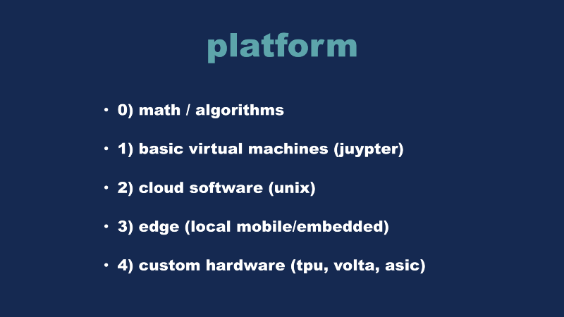
Very broadly, this is how I think about a lot of this stuff. At your most basic level, you have math and algorithms doing all this machine learning stuff. The next level up is basic virtual machines: Jupyter notebooks, stuff like that. The next level up there is cloud software, which is usually Unix in some form or another. You’re coordinating multiple machines and multiple GPUs to produce results. The next level up is the edge. This can be thought as taking cloud logic and running it locally in some form or another. The reason I think the edge is above the cloud is that often times with the cloud, you can sort of cheat against your problems. You can say, “Give me a server with a terabyte of ram.” And wham, your problem is solved. Whereas if you’re doing stuff on mobile devices, you often have very hard memory constraints, very hard processing constraints, and I think it’s another level of difficulty.

What this talk is going to be about is largely about custom hardware. We’re going to look at Google’s Tensor processing unit, the Volta architecture from Nvidia, and there are a whole bunch of machine learning startups and stuff out there right now. Some people are bringing custom ASICs to market in the next year or two. This is an area that’s very hot right now.

Getting Started with Machine Learning (3:30)

People sometimes ask me how to get started in machine learning. This is roughly how I think you should approach it if you were to start today. At the very least, you need to know Python. Python is basically the de facto language of machine learning right now. I included Roulette in the list. I think you need to have a basic understanding of statistics, but if I tell you to study statistics, you’ll go off and read a book about probability distributions and stuff like that and I don’t think that’s fairly practical. If you could go to Vegas and put a chip on the roulette table and you actually know what the odds are, that’s a good real-world understanding of probability and statistics.

In the same vein, you need to understand the basics of Calculus and linear algebra. I don’t think you need the full-blown Calc 3 college-level course, but you need to be thoroughly familiar with derivatives, integrals, and limits, things like that. I don’t think you need the advanced linear algebra either, but you really need to understand how to multiply matrices. The current course that’s the best way to go is the fast.ai 2018 sequence, this is all in PyTorch. I’ve been doing PyTorch a lot this last year, I’m a big fan of it. If you can do that course forward and backward, you can basically go out and go anywhere from there.

The next level up, you’ll have to start reading papers and other people’s code — we’re going to go through a bunch of papers here today. Then, you need to start practicing. Kaggle is good for this. What I tell people to do is to take on a Kaggle challenge from a year ago, because then you can go out and find other people’s code and see how they tried to solve the problems.

Finally, you need to get out into the real world. What’s exciting me about this whole field right now is that basically every person in this room has some problem that you understand better than everybody else, so you can take that problem and add a little bit of machine learning on top, and basically you can become the world’s main expert in that little niche. A lot of people make big deals about having PhDs and all this other stuff, and I think that’s completely the wrong mentality. I think everybody should be able to do this stuff.

JavaScript Warmup (6:10)

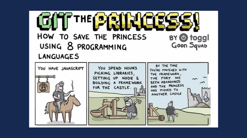
We’re going to do a little bit of JavaScript here at the start, just to get warmed up. This is a comic strip making fun of JavaScript for its ADD personality. The basic gist of my presentation I did a couple months ago was that JavaScript has this whole creative destruction element, it’s always changing and moving. I think that’s ultimately why it should be on your radar. Here are five demos with JavaScript that I will run through real fast here, illustrating some different concepts from the machine learning world.

TensorFlow.js: Train MNIST with the Layers API
I like this demo — whenever I show people CNNs, I always start with the MNIST dataset. I think that’s the best way to get going. This is just running in a browser, it’s running on MNIST. You’ve got your training curve, accuracy curve, and here at the end it’s going to show a whole set of data and it’s predictions. You can sort of see what the machine is thinking. It got these three right here, it predicted it was a 7, but it was a 3 that wasn’t drawn well. So you can kind of give the categorizer a little bit of leeway there.

ModelDepot
This is a demo that’s running the YOLO object recognition network on the browser against my webcam right here so you can see it trying to pick me up. It’s kind of a cool real-world example. It says I’m holding a cell phone in my hand instead of a microphone, but we don’t have everything trained perfectly.

Magenta.js
This is Magenta, it’s a project out of Google. I think it’s cool because a lot of machine learning stuff is oriented towards extracting another few percentage points of performance out of things, whereas this whole domain of art and computers is really interesting to me. It’s making some quasi-ambient IDM music here if you listen.

GAN Lab
This is a cool demo, it’s sort of visualizing how the GAN training process works, the distributions and how it learns them. This is something I don’t really have a good conceptual model of how it actually works, so I thought this was a cool way of looking at the whole thing. It has this button here that lets you restart it. I thought this was cool because you can see it introduce this cluster of pixels, and then slowly start stretching them out to map into the latent probability space. Cool stuff.

Mortal Kombat with TensorFlow.js
This is a demo I saw a couple weeks ago — I’m not going to run it for you, but they use transfer learning to learn gestures. You can shadow kick and fight and it controls a Mortal Combat character so you can shadow kick and fight with your friends just using a webcam.

TensorFlow.js Demo (9:50)

A couple of weeks ago, I did another talk on TensorFlow.js and I attempted to put together this demo. I didn’t quite get it working then, so I got it working last week. I thought I would show it off to you all. I’m not going to break down how it all works exactly, but if you wanted to look at the code, you can jump through the steps. Very broadly, we’re using mobilenets, which is a computer vision network. We’re using TensorFlow.js to run it. We combine all this code together into a docker/node container, and then we use IBM and OpenWhisk to upload it to the cloud where we can use it as a function. Then finally, I’m just running it locally by using a curl command, and then we Base64 code the image into a POST.

Here’s the actual command — just Base64 the picture, then we have this key and an API endpoint that everything runs against. We ran it on this picture of a bird that I have here locally on my computer, and it thinks that it’s an Indigo Bunting with an 85% probability. We’ll do it again, but with a panda picture. This one, it recognizes pretty well. It says we definitely have a panda, 99% probability. So that’s demonstrating different ways of doing machine learning problems by using a little bit of cloud magic, we’ll say.

Overview of Swift (12:15)

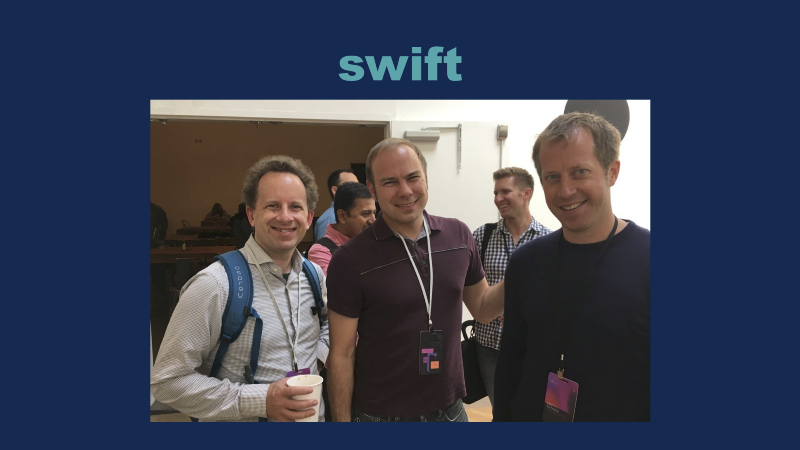
Now we’ll get into the meat of the presentation, we’ll do some Swift. This is a picture from the PyTorch developers conference earlier this year. I got to meet Chris Lattner. Very broadly, we’ll look at what a Tensor is, what we mean by a Flow, and what we get whenever we combine these two concepts together. We’ll review the current state of the art for image recognition training at scale, and then we’ll look at how I think Google is positioning LLVM and Swift to take things to the next level. In the end, I’ll try to give you a glimpse of where I think things will be at in the future.

So, what is a Tensor? I think a lot of people are comfortable with Matrix math and algebra, but I think whenever we combine these two concepts together, it starts to get a little bit fuzzy. Even this picture here, which I found on the internet, which shows that Tensor is a collection of Matrix objects, they’re not putting actual letters into here, like A, B, or C or whatnot and thinking about it in terms of properties as a whole.

You might take a linear equation, in the form of ‘Ax + B,’ then you can play games with it. You can make linear transforms. You can go from one transform to another, and if you start to build this up, you get a whole set of rules for combining rules and eventually you have a formal algebra for doing matrix math. This is a lot of work, but once you actually have the algebra, you can extend it with the algebra over graph and type theory.

Network Flows (14:05)

The big story of this last year or so and machine learning has been PyTorch and the concept of these network flows. The core concept is just that everything is fundamentally a directed graph, which means that if we can model the graph as a whole graph, and we only want to change one variable, then we can recompute just that one little thing that got changed as opposed to having to rebuild our graph the whole time. Google has wholeheartedly embraced this concept. Eager Execution is part of TensorFlow now for their TensorFlow 2 road map. That’s where they’re headed as well, so I think this is one of these key concepts that you need to know if you’re going to be working on this going forward.

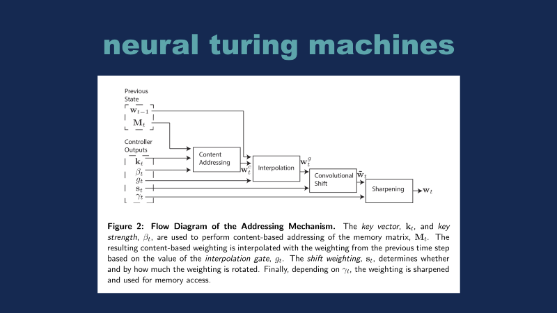
This is a paper from Alex Graves from a year or two ago. He built a formal architecture for modeling neural networks. What I think is powerful about this is basically you can think of all the neural networks and structures as being a combination of these blocks — you have your input data, you went through some sort of convolution and ‘Ax + B’ sort of steps, and you get your result, and you can think of a full-blown neural network as being a large collection of these blocks. You might take a thousand of these blocks and put them all together.

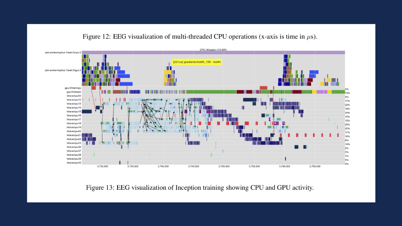
The reason why I think it’s important to think about this is that if you really look at the original TensorFlow paper, it’s not even really about GPU training per se as it is about this gigantic Gantt scheduler for performing these operations whenever you have a whole set of different things going on. It’s much less about the GPU per se as it is about coordinating across all these CPUs and getting the end result out of the time and doing so using the least amount of wall time, so to speak.

Faster Hardware (16:20)

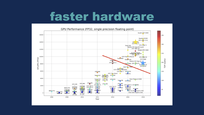
The second big story of the last decade or so is hardware. There has been this battle in the GPU space to improve things, and this is a cool graph because it basically has every single GPU from the last decade or so up here. What’s wild to me is that basically everything below the red line is now obsolete. That includes some Intel devices. I marked two of these devices with stars up here — this yellow star is the V100, the Volta, which we’ll talk more about in a second. This blue star is Nvidia’s new T4 GPU, which we’ll come to at the end. Just remember those for now.

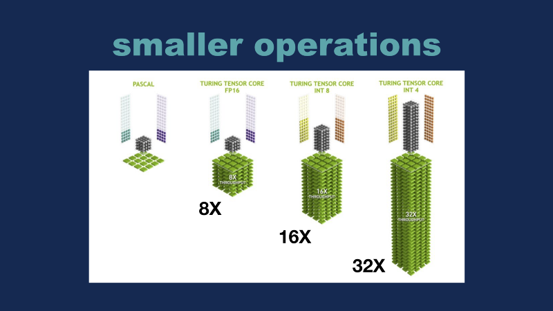
A random question — does anybody know where Google’s TPU would fit on this graph? It’s a trick question because the original TPU doesn’t do floating point 32 math, so it doesn’t even register on here. The reason I ask this question is that while I think most people conceptually can follow that hardware is getting faster and faster, the second piece of the puzzle for the last few years has been using smaller and smaller operations. If you go from a 32-bit floating point object down to a 16 bit one, and you can still do the same math, then that means you can do twice as many operations in the same time. The second trick is that they’ve introduced these various hardware devices (multiplier–accumulator) so that this whole step can be done even faster and faster. So we have the traditional floating point 32 bit here, we’ve got the floating point 16 bit, and the INT-8 which is what the original TPU was based around, which gives you a 16x speed up just by reducing the precision of math and finally we’ve got the INT-4 portion of the new Turing chips. Pay attention to FP16, because that is one of the important tricks that the Volta does.

High-performance Computing (18:55)

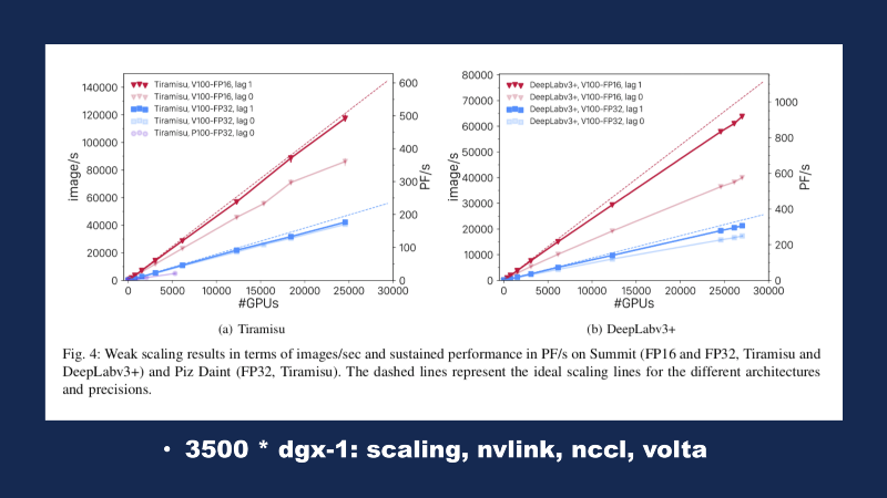
Next, we’ll jump over to the Summit supercomputer. This is at Oak Ridge, the former site of the Manhattan project, once upon a time. But nowadays, they do a lot of high-performance computing. This is the paper that came out last month on the summit supercomputer — they’re trying to model large climate systems using this computer, so the cool part of this graph is simply the x-axis. That’s 0 up to approximately 28000 GPUs being thrown at these problems. Then, what’s cool to me is that basically all of this work that’s gone into TensorFlow is basically linear scaling — the more GPUs you can throw at your problem, the faster you can get a solution. The Summit architecture is using a custom IBM architecture, there’s been a lot of work that’s gone on under the hood, very specifically with NVLink in order to deliver a unified memory architecture. The actual computer is not made of Nvidia DGX-1s, we’ll say, but you can think of this cluster as being roughly equal to 3 ½ thousand DGX-1s. If you’re on Amazon and you’re using a P3–16x Large, that’s a DGX-1, to give you a point of reference.

Most of us probably cannot take our problems and throw 20,000 GPUs at them, but all of us can take advantage of the difference between the red and blue lines here. The blue line is demonstrating FP-32 training, and the red line is demonstrating FP-16 training. These are two segmentation networks, but they modified the math to run on the lower precision operands, and so you can see that this one maxed out around 200 petaflops, but by reducing the precision of math, they were able to get to 500 petaflops. The same thing for this DeepLab over here, it maxed out around 300 petaflops using the FP-32, whereas whenever they went to FP-16, they were able to get up to somewhere in the range of 900 petaflops, honing in on that exaflop territory.

Converting your Models (21:45)

What do you need to do in order to convert your models from FP-32 to FP-16? Earlier this year, I took the Fast.ai course in person downtown and we worked on this DAWNbench competition out of Stanford. Our entry came in second in the Imagenet portion, and I can basically give you our high powered secret recipe for getting those results. Number one — algorithms. If you spend any time on anything, spend your time on algorithms. We had quantized hardware, we used Volta boxes (a DGX-1), and then we had quantized software. The PyTorch team upstream had done a lot of work in order to get Volta working on these devices, we had to do a bunch of coding in order to convert the Fast.ai code base to support the half-precision math, and then finally we did a little bit of distributed training on top by using 8 GPUs to solve each problem.

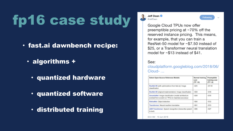
This picture is a little blurry, but it’s this guy at Google named Jeff Dean who was talking about how by implementing the algorithms that were introduced in the competition, they were able to reduce the cost of their training in half. That’s kind of cool.

For us, in order to implement all this, we basically had to do a lot of elbow grease. We did a lot of custom coding and whatnot. You all probably do not want to do that, and more broadly, that shouldn’t be what you have to do in order to get good performance out of your models. So about a decade ago, a company named Apple had a similar problem. They were locked to their GPU providers for their mobile devices, which is the iPhones. They wanted to change GPU providers, but they didn’t want to lose any performance for their existing code base, so they hired this guy named Chris Lattner and he came in and introduced LLVM. That’s a project he worked on at the University of Illinois. By doing this, they basically went from having to write a custom GPU code for every model that they needed to implement to just writing a way to get code into LLVM and another way for LLVM to get the code out for a specific GPU architecture. So then, adding new GPUs to their pipeline was simply a question of writing a new transpiler for that particular GPU.

As a direct result of this, they were able to switch their GPU manufacturers, but over time, many of these key concepts started to make their way into the larger iOS ecosystem. In the initial phase, they introduced Clang and LLVM into the Objective-C code base, and they started introducing memory and thread safety checks where the compiler can actually catch stuff long before it actually got pushed out into the field and would cause crashes there. They were retrofitting these changes on top of C, and they basically pushed it out about as far as they could. The next step was to introduce Swift and bring full-blown functional programming into the iOS world.

Something a lot of people don’t know nowadays is that you don’t even actually submit iOS code anymore. What you actually submit whenever you’re using XCode today is bytecode. It’s sort of a transpiled JIT sort of thing that you submit to Apple, and from there, Apple has servers that recompile your code for each individual device in the field to generate the optimized run time. So you push it up and they push down a different model for every single iPad or iPhone or so on. What’s wild about this approach is that if Apple comes up with a 10% improvement for coding optimization tomorrow, basically they can add that to their server fleet and recompile all the iOS code.

Tensor Comprehensions (21:45)

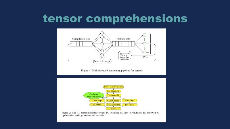
If you think about this concept, and you look at the Tensor comprehensions paper which came out of Facebook earlier this year, I think you can see that the GPU people are moving in the same direction. The top is illustrating the basic pipeline they have where they take GPU jobs, they run it through CPU or a cluster of some form, they profile the results and see if it’s better or worse than the previous one — if it’s better, they add it to their tuning database and they repeat the process over and over again. I think there will always be a spot for humans in the loop for this search strategy, but the other big story of the last year has been this introduction of evolutionary strategies in order to have computers improving the programs that the computers are running.

The second part down here at the bottom — this is a picture of how the Tensor comprehensions actually take input graphs and it generates optimized code. I think if you look at this and replace this green polyhedral transformation with TensorFlow and Swift, that’s basically what Google is thinking about introducing to the whole machine learning ecosystem.

In the same vein, even if you could generate a perfectly optimized model for your computer vision problem, in the real world you’ll probably be running your job on a cluster with other machines and other jobs, different devices. So it’s very easy for me to think, I take my job and run it at 80% of its normal speed, you take your job and run it at 60% of its normal speed, but the computer can find a way to combine these two jobs together to get two units of work in 1.5 units of time.

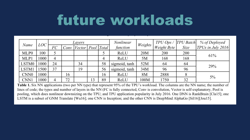
This is a graph from the TPU paper from Google a couple of years ago. What’s wild to me about this graph is this number over here in the bottom right corner, which is 5%. CNNs are pretty much what everyone thinks of whenever they’re thinking about neural networks. Very broadly, 95% of what Google does isn’t even CNN.

New TensorFlow and Swift Combinations (29:40)

What new capabilities will the TensorFlow and Swift combination unlock? A bunch of people are shipping new hardware to market in order to tackle these different problems. INT-8, as I mentioned before is part of the TPU — the new RTX cards have hardware for this. Then bfloat16 is a lesser-known data type, but it’s actually the native data type of the TPU-2s and TPU-3s. Intel is trying to bring hardware to market, and they are going after this data type as well. INT-4 is part of Turing, we’ll talk more about that in a second. There have been some academic papers that have been done on these. Binary networks, negative zero and positive were a big thing a couple years ago. This summer there was a paper called SignSGD which made heavy use of these Binary operations in order to reduce the communications between nodes to speed up distributed training, so that’s worth looking at.

People have gone all the way down to one-bit neural networks, so binary neural networks — Byte-net was a paper (2016) where they built up a language model using one-bit neural networks. It’s a very interesting approach.

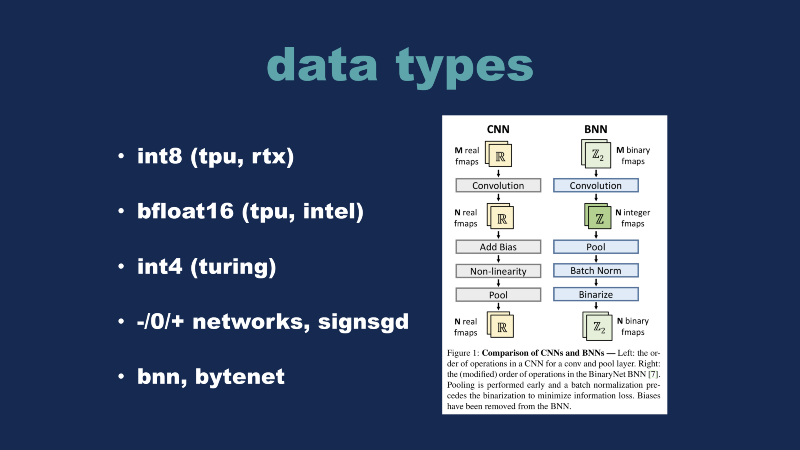
This graph is demonstrating a traditional CNN, you can simply think of a binary neural network as replacing all of the reals in the graph with integers. If you have a one-bit binary network, it’s a BNN. And if you have a two-bit binary network, it’s no longer a BNN, it’s referred to as a quantized neural network, or QNN. This graph gave me the idea for the demo I’m going to show in a second, this paper by Bert Moon in the Netherlands says that basically, they are able to target arbitrary model complexity or model size — if you have a very specific constraint, you can pick that and then you can work backward to how much error you’re willing to accept into your problem.

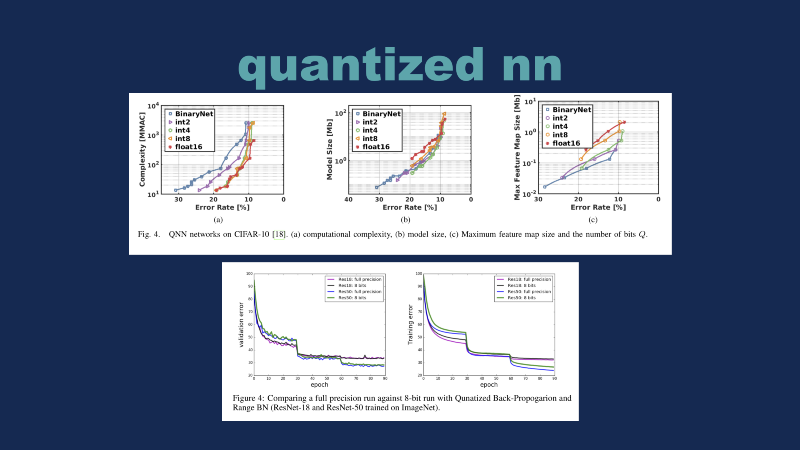
The second graph here — a lot of people are doing quantized neural networks, but they’re basically taking FP-32 models and simply converting the individual operands into integer math, so that they’re not technically training a quantized model that works, so to speak. This paper is very interesting because they introduce some tricks in order to have a stable loss and training validation curves for both ResNet and CIFAR.

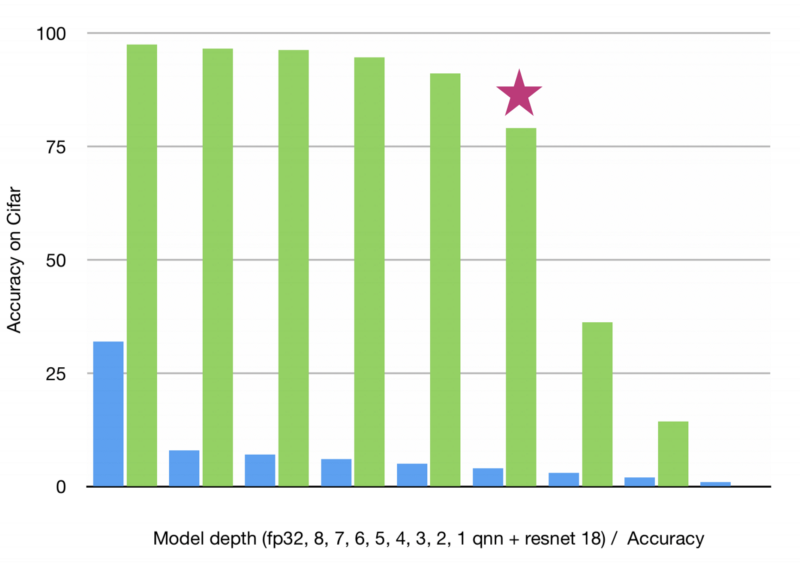
The demo I’m going to show is a demonstration of different QNN ResNet18 variants on CIFAR. We have our traditional floating point 32 model here on the far left, from there we work our way down from 8 bit, 7 bit, 6 bit, down to 1-bit models. As you can see, in each step, by reducing the amount of data we have available to the network, the accuracy of our network goes down slightly. Here our control has roughly 98% accuracy. We go to 8 bit, we go down to 97% accuracy. Each step, we lose a little bit more quality. On the flip side, if you go from 32 bit to 8 bit, we have a significantly smaller model. You lose a little bit of quality, but we have literally ¼ as large of a model and we can use this integer 8 math in order to run it even faster at runtime, which is very important for doing stuff on edge devices.

I didn’t write the code for this, a gentleman named Elad Hoffer did this demo. I simply modified his code to output these different results, and so we’re going to demo a 4 bit quantized ResNet18 running on the CIFAR dataset here.

Here’s my code, we’ll run it. I’m VPN’d into a Google Cloud box right here. It’s just a basic training loop for doing image recognition. If we run our nvidia-smi, we’ll see I’m running this on a Tesla T4 in the cloud. Google announced this about a month or two ago and I got an email that I was accepted into the Alpha program yesterday, so this morning I got this working, and so this may very well be the first T4 Google Cloud demo in the world. Shout out to them there for helping me out with that. If we let it run, it will keep on running for a while and it will end up with a network with around 80% accuracy, which really isn’t that great for CIFAR, but just remember that and we’ll come back to it in a second.

Recap (36:25)

Recap — we reviewed the current state of the art for hardware and software for doing image recognition and training. We looked at how people are moving from floating point 32 bit to floating point 16, and now people are starting to explore INT-8 models in order to speed up things even more. I talked about how I think Google is thinking about integrating LLVM and Swift into this whole thing in order to make this process simpler in the future, and then finally, we demonstrated a 4-bit QNN ResNet18 network training and running on actual 4-bit hardware.

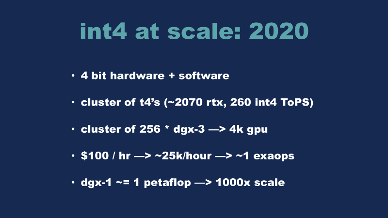
In the beginning, I promised to try and give you a glimpse into the future. Here’s my attempt to do so. I’ve shown you the hardware and software working together — all that exists here today, so let’s imagine that we have a cluster of these T4 GPUs. For real-world problems, it’s probably equivalent to the 2070 RTX, but they have about 260 TOPS for this INT-4 process here. Let’s imagine that we have a cluster of 256 DGX-3s. What is a DGX-3? Well, I just invented it. But a DGX-1 is a P3.16x large (8 Volta GPUs). DGX-2s are brand new, but they’re simply a 16 GPU version of the same. Imagine that we have 256 of these DGX-2s, we rip out the GPUs and we replace them with these T4 chips. Amazon charges you about $25 / hour for a P3 today, so let’s say that roughly speaking, this would cost you about $100 / hour. I think this may be on the high side, but it’s a reasonable number to work with.

So that would mean that for one hour, it would cost you about $25,000 to run this cluster. The end result is that you will have about 1 exaop of computational power to throw at your problem. If we think about a DGX-1 today as delivering roughly 1 petaflop, then in two years, roughly all of this stuff could be reasonably considered to be working all together. Conceptually, in two years, for the price of a decent used car, you’ll be able to afford as much computational power as currently the most powerful supercomputer in the world — if you’re willing to modify your algorithms to use the same form of math and if you can find a way to start working on getting that working now.

I started programming a long time ago in BASIC on a computer with a very small amount of RAM. To end this with a joke, I started out with an 8-bit computer, and now after all these years, I’ve moved on to a 4-bit computer. Thank you all for coming. The links to the demos and sources to the papers will be included.

P.S. Thank you to James Maki for giving me feedback on this speech!