
A presentation for the Advanced Spark and Tensorflow Meetup (thanks Chris Fregly!) at Grammarly about different approaches used on SQuAD for the Dawnbench competition.
Video • Slides
Introduction (1:20)
About a year ago, they had the Stanford Dawnbench competition. There were two computer vision problems, and then an NLP (natural language processing) problem. At the time, I wanted to work on the NLP part, but I didn’t really have the time and resources to go after it. Then late last summer, they decided to have rolling submissions, so people could submit new results. So, I started working on this problem again. Historically, I’ve done a lot of computer vision stuff, but I’ve not done a ton of NLP. So, this is a good problem for me to really go deep into NLP, it’s kind of new territory for me. As a result, I’ve learned way too much about this SQuAD problem. So I thought I would share some of the stuff I’ve learned as a jumping off point if anybody else is interested in this field.
Overview (1:22)
At a high level, we’ll look at this SQuAD problem itself and we’ll look at the seq2seq paper, which I think is the basis in most of these approaches. We’ll look at four different methods of solving the SQuAD problem, and each of them were state of the art at some point in time or another, so we’ll look at how each one works and what makes them different. From there, we’ll jump over to look at version 2 of the SQuAD dataset, which is a very hot modern area of NLP research with a whole bunch of people competing on this. Then we’ll look at the stuff that builds up to the BERT paper which came out last fall. It’s pretty close to the current state of the art for this field. At the end, I’ll try to leave you with some next steps and where to go from here.
The SQuAD Problem (1:24)
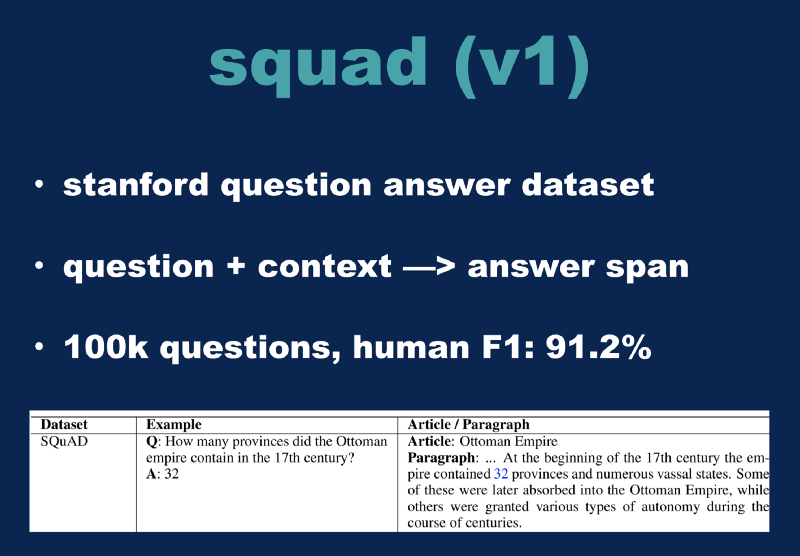
The SQuAD problem — it’s quite simply an acronym for Stanford Question Answer Dataset. They have a large collection of Wikipedia articles with questions that are associated, and then you’re supposed to identify the span of data that is the answer of the results. So right here at the bottom of the screen is an example of what a Wikipedia article would look like, what a question would look like, and you’re supposed to identify the answer 32. There are about a hundred thousand questions in this dataset, and the human’s F1 score is about 91.2%.
 Stanford Question Answer Dataset
About Seq2seq (1:25)
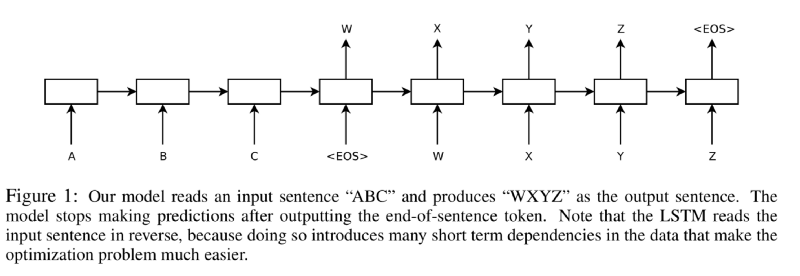
Seq2seq — this is an older paper, but I think it’s the basis of a lot of modern NLP approaches, so I thought it was worth looking at. The key idea is that we combine both our input and our output, as our input. Then, we tie it together to the contextual answer. So, the classical example of this would be a translation. So, we take a sentence in one language and combine it with its pair in another language, and then try to train our neural network to recognize the result that we’re looking for in the other language. There are a couple of different ways of thinking about this, but I like to think about it as a data augmentation technique almost. We’re giving the machine more data so we can make it easier to learn the right results.
 seq2seq
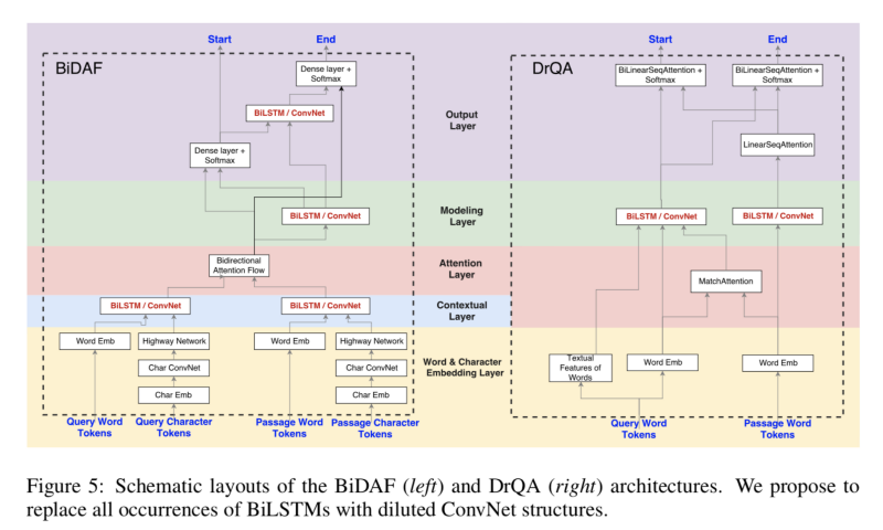
To continue this, when people think of seq2seq, usually it’s in the context of inputs. But you can also think of each of these A, B, and C, and W, X, Y, and Z outputs as being an entirely different input. We might concatenate several different inputs together, in order to produce our end result. If you think about it like this and then look at the bi-directional attention flow paper, which was one of the first state of the art approaches to the SQuAD problem, I think you can see the same basic idea. If you look down here at the bottom, you can see a combination of different word embedding layers. So if you have two different word embeddings, one for using the traditional GLOVE word embedding vectors. Then they’re also using the second one on the raw character data, so they use the Char-CNN. They combine these two results as their context, and then they combine them with the query or the question, the result they’re looking for. They run it through an attention model, and then this BiDirectional LSTM in order to produce the final output. This is a little bit older of an approach, but it’s the same concept as the basis of the other approaches we’re going to look at here.
Looking into DrQA (1:27)
The next one we’ll look at is DrQA. This is a paper out of Facebook from a couple of years ago. The crucial difference between this one and the BiDAF is that we’re adding one more input layer, which is the document metadata itself. This means that within the attention network at the end, it has a context of the right Wikipedia articles to be looking into. This, by extension, improves the results. This particular slide is from a different paper that I was looking at. I liked that they compared in contrast the BiDAF on the left with the DrQA models. Basically DrQA is a little bit simpler, but actually produces better results.
 BiLSTM vs DrQA models
If you take this idea of adding more data to the model to its logical conclusion, then we might literally add a half dozen layers worth of potential information sources and then use the neural network to try to make sense of it all. This is Fusionnet, it’s actually an older paper from 2016. But they utilize this approach in order to produce even better results than the two models that I’ve shown you so far. The problem with this is that we’re adding so much data to our network that the end result is starting to go pretty slow. Then, the FusionNet people added on top, this simple recurring unit — if you’re familiar with RNNs and unrolling RNNs, I would think of this model as basically as conceptually unrolling the RNN into something kind of like a CNN style approach. The practical upshot of this is that they have something they can train much faster and simpler than the traditional BiDirectional LSTM approach.
Then if we take this idea and go one step further, we might build an entire full blown CNN style residual block approach for our data. This is basically how QANet works. This is a paper out of Google from last year around May 2018. I would argue that the CNN approach isn’t as powerful at detecting as the LSTM approach, but because it’s a CNN approach, it can be made bigger. This model can be made much larger than the LSTM approaches we’ve been seeing before, and as you’ll see here in a second, that allows it to scale up and produce even better results.

Here’s the Dawnbench leaderboard as of the start of last month. We can see all these different approaches I’ve shown to you. Each one was at one point or another the state of the art in this field. On the left side, I have what, under perfect conditions, these networks were trained to, roughly. So the BiDAF will get up to around 76% if you give it a significant amount of CPU time. DrQA can get around 78% for an F1 score. The FusionNet plus the SRU approach does even better at around 82%. And finally, QANet can be trained up to around 84% for the SQuAD problem. I’ll have you look over here at the third column over — this is the time that each approach is taking. So the original BiDAF approach running on an old K80 took about 8 hours to run. The DrQA is roughly an order of magnitude simpler, it runs somewhere around an hour. The official GoogleNet Google submission for QANet is 45 minutes. We’ll come back to that one here in a second. Then last month, the FusionNet plus SRU, which they labeled as FastFusionNet was able to produce a .75 F1 score in under 20 minutes. I attempted to get each of these running for you. All the code for the BiDAF was like Pytorch 0.3 era stuff, and relied on older versions of CUDA, so I tried to bang on that for a while, it didn’t have much luck. I’ll demo DrQA running on a T4, the exact same machine that’s the fourth place result up here. I attempted to get the FusionNet and SRU code working, but I had some difficulties with that. Then we’ll also demo QANet running on a TPU here.
Okay, I’m VPN’d into my Linux box. This is my DrQA box running right here, so we’ll just fire it off. We’ll come back to this one in a second. We’re going to run the QANet on a TPU, so I spun up the TPU earlier. That command looks like this, right here. This is what the actual code to run the TPU job looks like. The QANet is a little bit weird, but basically, I have to have one process running the evaluation loop — that’s this command right here. Then I have a second process that’s going to be running the actual training of the QANet. We’ll fire up the evaluation script right here. So now it’s basically running and waiting. We’ll remember this number right here, 3 hours and 14 minutes. Then right here, we’ll run the actual QANet training code. Then we’re also going to run it with just one epoch. It’ll get going right here… Here we go. Let’s save this time here just as a checkpoint. So at 3 hours, 15 minutes, we started this job.
Second Generation of SQuAD (1:36)
Now we’ll look at the second generation of SQuAD. The problem with the SQuAD is that these neural networks will overfit the results, so what happens is that you can give it an adversarial question, and the network will find answers that are basically nonsensical. So what they did is they added 50,000 human generated questions that are designed to all have negative answers. So this makes the problem significantly more difficult, because not only does the network now have to find the answer, but it also has to know when the answer is not actually in the data. This area has been an area of very competitive research, a number of NLP researchers in Asia are going after this, as well as the Google team. This is the leaderboard for SQuAD 2.0. The crucial thing to note about this leaderboard is that each of these entries has the word BERT up here. BERT is a new NLP model that came out last fall. So now I’m going to spend a little bit of time breaking that down. But as of the last week or two, these models have started to approach human levels of performance in this field, and I think they’re going to rapidly improve from here.
The first important concept you should know is this idea of this transformer model. I think of this as taking the seq2seq model from before and making a formal version of it wherein by you can take any combination of input data, and you can map them together using roughly the same concepts, but using much more CPU cycles, though you also get much better results.
The second important concept to add on top is this concept of transfer learning or pre-training as it’s sometimes referred to. This is a very common technique in the computer vision community, but historically, it has not been very popular within the realm of NLP. Basically, we can take a network, and train it on one problem. In computer vision, we train on ImageNet, and then we apply it to a different problem such as recognizing people’s faces. This works very well in computer vision, but it has not had a lot of success for applying it to NLP until the middle of last year when the ULMFiT paper came out.
This is Jeremy Howard with FastAI. They did this paper where they trained a three-layer LSTM model on the Wikipedia data set, and then on graph C, they were able to unfreeze the final layer, and then retrain it or fine tune it on to a different problem and produce state of the art results in this field. So this paper came out and it generated a lot of attention. As a result, the Google team basically took this idea and ran with it and produced the BERT model.
 BERT vs GPT vs ELMo
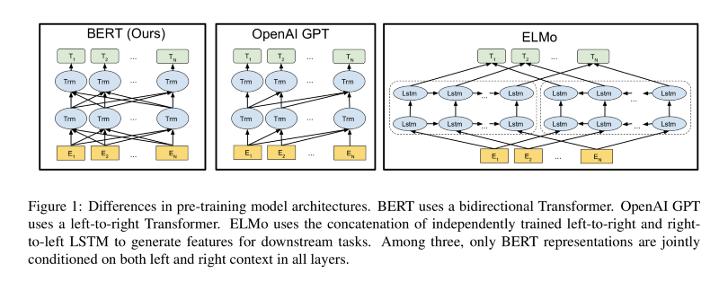
The BERT model uses a BiDirectional transformer model. This can be thought of as being similar to the BiDirectional LSTM, but instead, we’re replacing the LSTM modules with transformer modules. There are a couple of other variants of this out here, they’re shown up here. The ELMo model has two LSTM networks that are overlaid, but they don’t technically talk to each other. OpenAI’s GPT model is using a directional graph that always goes to the right. There are some interesting properties of this because you can make it larger. But basically, BERT uses a large collection of these attention layers and a large collection of these transformer heads in order to produce state of the art results for doing NLP problems, as well as being trained on Wikipedia to start with. So this was significantly computationally expensive to build this model, though there’s been some recent progress in that area as well.
What we’ll do now is look at one more demo, and then we’ll see if our QANet has had any luck. There’s this company called Huggingface that develops AI chatbots. They have a very nice set of demonstrations of Pytorch code running a handful of different NLP models that you can download. I have their BERT model running in a virtual machine, and then we’ll just fire it off and we’re going to retrain it on this SQuAD dataset in the cloud using a T4. We’ll give this a second or two to get going here. Now it’s running. It will take about 2 hours to do each iteration, and then we run it for two epochs over the dataset. This particular run will take about 4 hours to run. Now let’s go back to the QANetwork… Here is our QANet results from running it for a little bit. We’ve evaluated to an F1 score of .76, and we’ve run through approximately 20,000 global steps. This means that it’s actually gone through the equivalent of 6–7 epochs of the other Dawnbench models, but basically, we trained from 0 up to .76 F1 in a little over 10 minutes. This is even faster than the current number 1 leader on the Dawnbench leaderboard.
Conclusion (1:44)
To wrap it up, I’ll leave you with three different ways to tackle the SQuAD problem. The first one is the retrained BERT. This will get up to an 88% F1 accuracy, which is better than any of the models I’ve shown you before, and it can be done in about 4 hours on T4, which means it would cost you about $5 to run. The second method is this QANet running on a TPU2, which will get you to a .75 F1 score in about 10 minutes. That’s twice as fast as the current leader on the leaderboard. For simplicity, I still think the best approach is this DrQA model — Runqi Yang wrote the original model and I modified it slightly in order to produce these Dawnbench results, but I would highly suggest that you check out his work. Then the future stuff that we’re looking at — Transformer XL came out recently, this is a larger version of the transformer model, which Google has worked on scaling it up to train it on larger and larger clusters, and then OpenAI has released GPT and recently GPT-2, these are also very interesting NLP models that you should look at. Then finally, there is this other competition out there called MLPerf which I think is worth investigating if you’re interested in these benchmarking training results.
There you go, and thank you all for coming! Any questions?
Questions & Answers (1:46)
Q: Did you re-implement all of these models, or are they open sourced that you just used, or a mix of both?
A: This is the DrQA model right here. You can download it. QANet is part of Google’s TPU examples. I’m just running this whole demo right here. I modified this 1 to be a 5 to make sure that it stopped at the right spot for the demo. Here’s the actual SQUaD leaderboard, if you’re interested in keeping track where the current state of the art is in this field. Here is the Huggingface Pytorch pre-trained BERT, they have other models as well. But here’s the actual SQuAD code that I just ran. Then everything I’m doing right here is just being done on a collection of virtual machines and the Google cloud platform, plus one TPU over here.
Code
Papers
Background: seq2seq, squad v1, squad v2, glove, char-cnn, pretraining
Optimizations: fast reading comp, sru, lamb
Models: bidaf, drqa, fusionnet, qanet
Advanced models: transformer, ulmfit, elmo, gpt-1, bert, transformer-xl, gpt-2